Kubernetes Resources Overview

​

Overview

Chalk’s metadata and data planes can both be deployed to Kubernetes clusters running in your cloud. This page provides an overview of the Kubernetes resources used by Chalk, so that you can understand how to configure, monitor, and troubleshoot your Chalk deployment.

​

Metadata Plane

The Metadata Plane is responsible for storing and serving non-feature data (like alert and RBAC configurations). It orchestrates machines in the Data Plane using the Kubernetes API to do things like scaling deployments, and running batch jobs.

The metadata plane currently consists of the following primary kubernetes components:

• go-api-server: presents a gRPC interface for driving orchestration.
• api-server: presents a REST and GraphQL interface for driving orchestration.
• frontend-server: This is a web application that serves the Chalk UI.
• Cluster Ingress: Either Envoy, Amazon Application Load Balancer, or Google Load Balancer. This routes traffic to the API server and frontend server.

You may deploy these components yourself using a helm chart, or Chalk may manage the deployment as part of our standard Customer Cloud deployment model.

Typically these components do not scale with you query volume and represent a roughly fixed cost. Most online query traffic will not flow through these components — it will flow directly to the data plane.

​

Data Plane

The Data Plane consists of components that execute your feature pipelines, your online store, and your offline store.

The data plane currently consists of the following primary Kubernetes components:

• engine deployments: These are feature pipeline execution engines. These pods execute your Python code in Chalk’s execution environment.
• engine-grpc deployments: Same as engine deployments, but with a gRPC interface. Query semantics are the same, but the network runtime is C++ instead of Python.
• branch deployments: A stateful set or deployment object that runs your branch deployments.
• job kubernetes jobs: These are batch jobs that run your Python code in Chalk’s execution environment for scheduled tasks.
• query job kubernetes jobs: These are batch jobs that run your Python code in Chalk’s execution environment for async offline query tasks.
• streaming statefulset: A stateful set that runs your streaming deployments. These are long-running processes that consume from a message queue and write to the online and offline store.

​

Configuring Data Plane Resources

The Data Plane is the component that scales with your query volume. Each component in the data plane can be configuring via the Settings -> Resources page in the Chalk UI. The key scaling dimensions are:

• replica count: The number of pods that will be running for a given service
• CPU and memory requests and limits: The amount of CPU and memory that each replica will use

Depending on your workload, you may want to scale different components in the data plane in different ways.

​

Online Query Scaling

The online query path is typically the most critical component in Chalk. It is the component that your application will use to query features in real-time. This workload is served by the engine and engine-grpc deployments. These deployments are stateless and can be scaled horizontally to handle more query volume. The key scaling dimensions are:

• replica count
• CPU and memory requests and limits

Horizontal scaling is achieved via autoscaling. min_instances and max_instances are set in the Chalk UI, and the autoscaler will scale the number of replicas based on the query volume. Simple CPU-based autoscaling is supported out of the box via the “Target CPU %” setting, and more advanced autoscaling can be achieved by setting up custom KEDA scalers, controlled via the JSON field in the Chalk UI.

Different query workloads require different ratios of CPU and memory. The engine and engine-grpc deployments have a resources section in their deployment spec that can be customized to match your workload. Typically, workloads which execute more Python code will require more CPU. Workloads which have a smaller working set of data will tend to scale more efficiently with more small replicas, while workloads with a larger working set of data will tend to scale more efficiently with fewer larger replicas.

​

Configuring Online Query Parameters

Chalk recommends setting scaling parameters by running realistic query workloads and monitoring the performance of your queries. The Overview page in the Chalk UI reports CPU and Memory utilization metrics for your online queries, and you can use these to tune your resources appropriately.

If you see high CPU utilization, you may want to increase the CPU requests and limits for your deployments, or increase the number of instances. For optimal tail latency, you may wish to maintain CPU significantly below 100%. If you see high tail latency and low cpu utilization, contact Chalk Support — you may need to tune your Python code or configure thread pools or connections pools.

A given set of configuration for a deployment will support a particular query volume. If you see high latency or high error rates, you may need to scale your deployment up or out. If you see latency that increases with query volume, you may have an underscaling problem that is causing request queueing.

​

Offline Query Scaling

The offline query path is typically used for training models, generating training sets, and other batch processing tasks. This workload is served async offline query jobs. These jobs consume no resources while they are not running, because Kubernetes Job objects are used to run them. The key scaling dimensions are:

• CPU and memory requests and limits
• num_workers parameter to the offline_query method
• num_shards parameter to the offline_query method

The num_workers parameter controls the number of parallel workers that will be used to execute the query. The num_shards parameter controls the number of shards that the query will be split into. By default, num_workers = num_shards, and this is a good starting point for most workloads. However, you may want to increase num_workers to horizontally scale your workload. You may want to use more shards if you experience memory pressure and the working set is easily partitionable.

You should tune your resources section in the offline_query method to match your workload. The Offline Query details page reports CPU and Memory utilization metrics for your offline queries, and you can use these to tune your resources appropriately.

Typically, we recommend increasing CPU if you see high CPU utilization, and increasing memory if you see out-of-memory errors.

​

Workload Isolation with Resource Groups

Chalk supports workload isolation via Resource Groups. Typically, resource groups are used to isolate workloads that have different scaling characteristics, different cost accounting requirements, or to ensure limited blast radius in service of production resilience.

Resource Groups allow you to specify isolated node pools for different workloads. For example, you may want to run your online query workload on a separate node pool from your offline training workload. This can be achieved by setting up separate Resource Groups for each workload and specifying the resource_group= parameter for offline queries, and the query_server parameter for online query ChalkClient instances.

More advanced configurations are also possible. Chalk Support can assist in routing traffic by query_name, or by random sampling for experiment workflows.

​

Other Components

cluster ingress: The cluster ingress is a component that routes traffic to the metadata and data planes. It is typically deployed as a separate component from the metadata and data planes, and is responsible for routing traffic to the correct component based on the request path.

Typically, you will not need to scale this component. Monitoring it can be useful to ensure that there are no HTTP or gRPC layer errors.

metrics database: The metrics database is a component that stores metrics data for Chalk. Typically, this is a TimescaleDB instance, and one is deployed per Chalk environment. The metrics database is responsible for storing information and metrics about queries run in a Chalk environment. For self-hosted deployments, you should monitor disk usage in the associated persistent disks.

background persistence: The background persistence component is responsible for persisting batch, streaming, and online query results to the online and offline stores. This component also computes value metrics and persists them to the metrics database. This component uses KEDA to autoscale queue consumers, and is not typically manually scaled. Error logs from this component can be useful for diagnosing issues with query persistence. Issues typically do immediately impact online query performance, but can impact the ability to generate training sets or certain caching workflows.

​

Concrete Scaling Choices

​

Production Environments

In production environments, we recommend the following scaling choices:

• engine and engine-grpc deployments:
  • >= 2 replicas, with CPU and memory requests and limits set to >= 2 core and >= 4 GB of memory
  • Memory needs to be proportional to the number of UDF invoker processes you choose to use
  • If you choose to use a single replica, you will experience query downtime (502s, UNAVAILABLE responses) during pod restarts.
• query-job:
  • set to >= 8 cpu and >= 16GB of memory
• streaming:
  • use >= 1 replica, with a low cpu request (i.e. 1-2)
  • set a cpu target of 80%

​

Scaling under workload

​

CPU Scaling

CPU scaling is typically the most important scaling dimension for online queries, contrary to what you might expect you should not choose target cpu > 50% for the scaling target if latency is important.

Queueing Theory proves that:

• The average response time of a system is proportional to the utilization of the system
• The specific formula is:
  • T = (1 / (1 - U)) * (1 / mu)
    • T is the mean response time
    • mu is the service rate of the system (# of reqs/sec the system can complete at 100% cpu)
    • U is the utilization of the system (arrival rate / service rate)

Working this example for a few values of T:

• At 40% utilization, the average response time is 1.7x the service rate
• At 50% utilization, the average response time is 2x the service rate
• At 80% utilization, the average response time is 5x the service rate

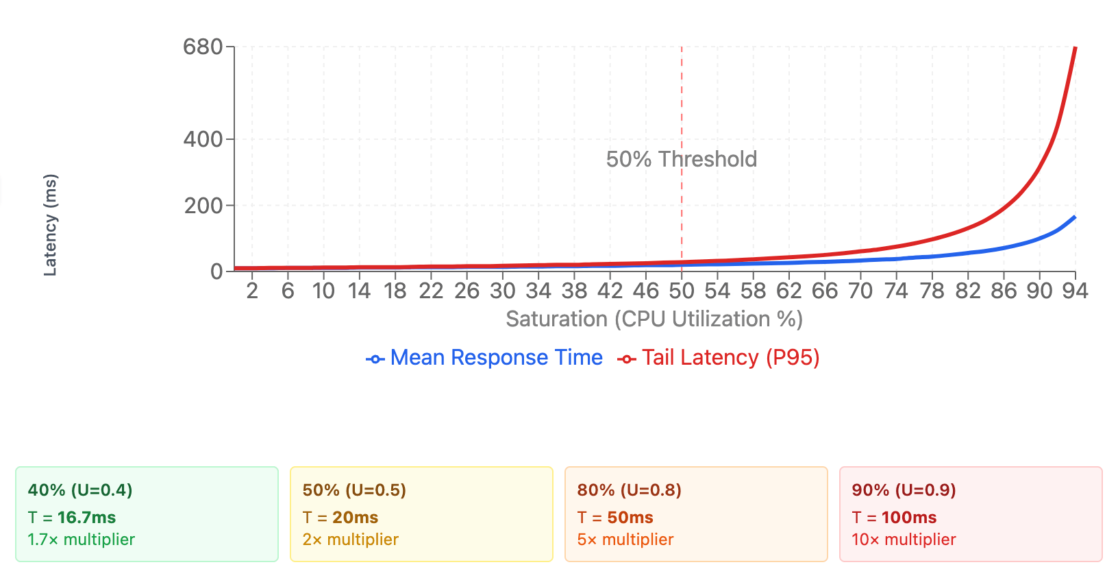
The theory shows that latency increases superlinearly with CPU utilization, and this is especially true for tail latency. This means that if you set the target CPU to > 50%, you will see a significant increase in tail latency.

​

Rate limiting

Servers have a finite capacity for concurrent processing. When incoming request volume exceeds the ‘clearing’ rate of the server, the server will queue requests. This can lead to increased latency and errors. In particular, if the requests need to be completed by a particular time, the server will (naively) waste resources processing requests that will not complete by the deadline.

To mitigate this, Chalk supports rate limiting for the engine-grpc component. The engine-grpc component supports these environment variables to establish concrete rate limits:

• CHALK_GRPC_RATE_LIMIT_TYPE
  • noop: default; no rate limiting
  • concurrency: limit the number of concurrent queries
  • qps: limit the number of queries per second using a token bucket rate limiter
• CHALK_GRPC_RATE_LIMIT: The number of concurrent queries or queries per second that should be permitted.

Typically, we recommend that using the qps rate limiting option for standard workloads, and concurrency for latency-sensitive workloads.

​

Node pools:

• Configure isolated node pools for online query workloads and offline query workloads
• Use the chalk.ai/workload-class taint to prohibit workloads from scheduling on the wrong node pool

Node pool isolation means that you can run offline queries concurrently with latency sensitive workloads without impacting the performance of the online query workload.

​

Select a machine type:

It is often useful to select a specific machine type for certain Chalk workloads in order to guarantee that those workloads run on a high-performance cpu architecture, have a particular ratio of memory to cpu available, or run isolated on individual machines.

​

AWS

Chalk deployments in AWS EKS clusters use Karpenter to provision nodes (cloud machine instances) for workloads. In order to specify an instance type, add a node selector to a Chalk service kind in Settings > Resources > [Service Kind] > Advanced > “Kubernetes Node Selectors” with the key node.kubernetes.io/instance-type. The value should be the name of the desired EC2 instance type.

For example, if you would like your query servers to run on c7i.4xlarge instances, set the node selector node.kubernetes.io/instance-type: c7i.4xlarge.

​

GCP

Chalk deployments in GCP GKE clusters use either GCP node auto-provisioning (NAP) or manually-configured GKE nodepools to provision nodes for workloads.

When using NAP, the “machine family” can be specified via a node selector in Settings > Resources > [Service Kind] > Advanced > “Kubernetes Node Selectors” with the key cloud.google.com/machine-family. The value should be the name of the desired machine family. For example, if you would like your query servers to run on c3d instances, set the node selector cloud.google.com/machine-family: c3d.

When using manually-configured GKE nodepools, the nodepool for a workload can be specified by name with the node selector cloud.google.com/gke-nodepool. For example, to run workloads on a nodepool called chalk-c3d-standard-4-nodepool, use the node selector cloud.google.com/gke-nodepool: chalk-c3d-standard-4-nodepool.

GKE nodepools cannot currently be configured in the Chalk dashboard, so they must be configured via the GCP console.